Selected segmentation methods
In this section, we will introduce 3 selected segmentation methods: SLIC, activecountour and lazysnapping. With SLIC, we will use the concept of superpixels and it is fully automatic. Activecountour and lazysnapping are methods for which assistance is suitable, i.e. approximate marking of foreground and background is desirable.
In image segmentation, the term superpixel is used in several methods. A superpixel is an area of points in the image with similar properties, while it should be more meaningful from the point of view of perception than individual points of the image. A well-known algorithm for dividing the image into superpixels is SLIC (Simple Linear Iterative Clustering) [1]. SLIC is a modification of the K-means algorithm, which we previously mentioned in color image segmentation.K-means formed clusters based on the similarity of the values of the image points in the color space, regardless of their position. SLIC extends K-means by position information, so instead of looking for similarities in a 3-dimensional color space, we look for similarities in a 5-dimensional space. I.e. coordinates are \((R, G, B, x, y)\), or in another color space \((H, S, V, x, y)\) and so on. SLIC algorithm takes into account that in this 5-dimensional space two types of coordinates, spatial and value, are combined, so it calculates "color" and spatial distance separately. These distances are subsequently normalized and weighted into the resulting distance. Using the weight, it is possible to determine the importance of the color and spatial component in the resulting distance. In the MATLAB environment in the superpixels function, this is included in the "Compactness" parameter. An example of creating superpixels is shown in Fig. 1. We can see that, with 2 superpixels, he has excellently separated the foreground from the background.

Fig. 1 An example of creating superpixels with the SLIC algorithm
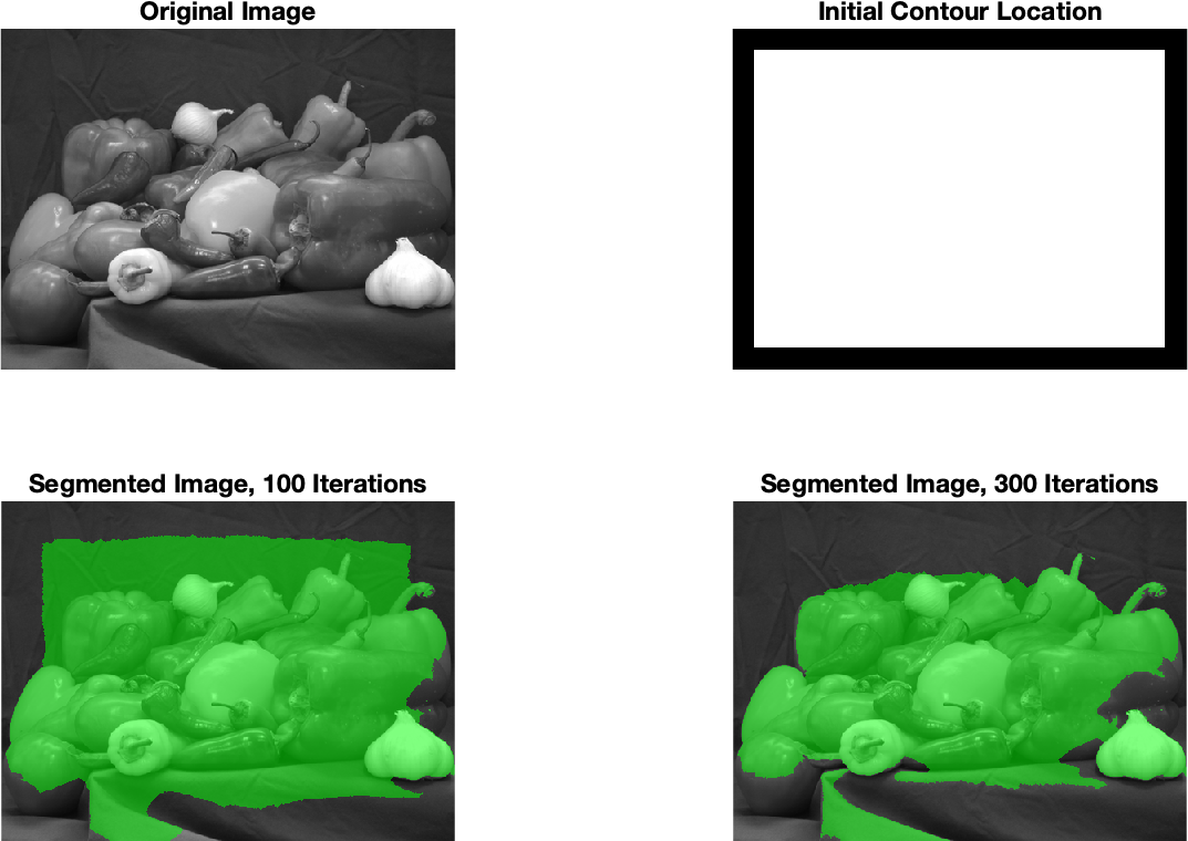
The activecontour method uses the initial roughly drawn contour (boundary) of the foreground object and tries to refine it. Several refinement algorithms are implemented in the MATLAB environment. The Chan-Vese algorithm [2] can be used for the color image, which is based on the evolution of curves (area boundaries) with the criterion of minimizing the metric based on the weighted energy of the regions and the overlap with the current area. The evolution takes place during a specified number of iterations. An example of application and the obtained result is shown in Fig. 2.
The lazysnapping method refines (snapping) to a roughly sketched background and foreground. The original article [3] used curves, the MATLAB implementation uses areas. The method is based on graph theory and cuts in network graphs with energy minimization. It uses superpixels instead of pixels. An example of application and the obtained result is shown in Fig. 3.

Fig. 2 Example of segmentation using the activecontour method with the Chan-Vese algorithm

Fig. 3 An example of segmentation using the lazysnapping method
References
[1] Radhakrishna Achanta, Appu Shaji, Kevin Smith, Aurelien Lucchi, Pascal Fua, and Sabine Susstrunk, SLIC Superpixels Compared to State-of-the-art Superpixel Methods. IEEE Transactions on Pattern Analysis and Machine Intelligence, Volume 34, Issue 11, pp. 2274-2282, May 2012
[2] T. F. Chan, L. A. Vese, Active contours without edges. IEEE Transactions on Image Processing, Volume 10, Issue 2, pp. 266-277, 2001.
[3] Y. Li, S. Jian, C. Tang, H. Shum, Lazy Snapping In Proceedings from the 31st International Conference on Computer Graphics and Interactive Techniques, 2004.
Appnedix
The source code of the program that created Fig. 1
clear all; close all; clc;
fig=figure;

subplot(3,2,1)
RGB = imread("peppers.png");
imshow(RGB)
title("Original Image")

N=[2,5,10,50,500];
for idx=1:size(N,2)
    subplot(3,2,idx+1)
    L = superpixels(RGB,N(idx));
    BW = boundarymask(L);
    %imshow(imoverlay(RGB,BW,'cyan'),'InitialMagnification',67)
    imshow(imoverlay(RGB,BW,'cyan'))
    title(sprintf("%u Superpixels overlay",N(idx)));
end

fig.PaperUnits = 'inches';
fig.PaperPosition = [0 0 10 10];
print(fig,"segmOtherClic.png",'-dpng');
The source code of the program that created Fig. 2
clear all; close all; clc;
fig=figure;
subplot(2,2,1)
I = im2gray(imread("peppers.png"));
imshow(I)
title("Original Image")

subplot(2,2,2)
mask = zeros(size(I));
mask(25:end-25,25:end-25) = 1;
imshow(mask)
title('Initial Contour Location')

subplot(2,2,3)
bw = activecontour(I,mask);
imshow(labeloverlay(I,bw,'Colormap',[0 1 0]))
title('Segmented Image, 100 Iterations')


subplot(2,2,4)
bw = activecontour(I,mask,300);
imshow(labeloverlay(I,bw,'Colormap',[0 1 0]))
title('Segmented Image, 300 Iterations')

fig.PaperUnits = 'inches';
fig.PaperPosition = [0 0 10 6];
print(fig,"segmOtherActivecountour.png",'-dpng');
The source code of the program that created Fig. 3
clear all; close all; clc;
fig=figure;
subplot(3,2,1)
RGB = imread("peppers.png");
imshow(RGB)
title("Original Image")

subplot(3,2,2)
L = superpixels(RGB,500);
 BW = boundarymask(L);
%imshow(imoverlay(RGB,BW,'cyan'),'InitialMagnification',67)
imshow(imoverlay(RGB,BW,'cyan'),'InitialMagnification',67)
title("Superpixels overlay")

subplot(3,2,3)
imshow(RGB)
f = drawrectangle(gca,'Position',[100 128 350 150],'Color','g');
foreground = createMask(f,RGB);
b1 = drawrectangle(gca,'Position',[130 30 40 30],'Color','r');
b2 = drawrectangle(gca,'Position',[6 368 500 10],'Color','r');
title("Background/foreground marked")

subplot(3,2,4)
background = createMask(b1,RGB) + createMask(b2,RGB);
BW = lazysnapping(RGB,L,foreground,background);
imshow(labeloverlay(RGB,BW,'Colormap',[0 1 0]))
title("Lazy snapped image")

subplot(3,2,[5:6])
maskedImage = RGB;
maskedImage(repmat(~BW,[1 1 3])) = 0;
imshow(maskedImage)
title("Background changed to black")

fig.PaperUnits = 'inches';
fig.PaperPosition = [0 0 10 12];
print(fig,"segmOtherLazysnapping.png",'-dpng');
The PDF version of this text is available here: segmentation_other_eng.pdf