Color image segmentation and K-means
When segmenting a color image using thresholding, we can apply thresholding separately to each color channel. Alternatively, we can transform the image into another color space and perform the thresholding there. Since thresholding is a non-linear operation, the results will be different. It is necessary to choose a suitable color space if we want better separate the individual classes from each other. When thresholding color images per color channel, in 3D we can interpret the values defined by the thresholds for the object in the foreground as a cuboid. By changing the thresholds, we just move the positions of cuboid walls. With manual methods, we move the thresholds manually, with (semi)automatic methods, we move them (semi)automatically.
K-means clustering is representative of methods where the boundaries between classes can be more complicated (not just linear walls). In the case of K-means, we search in \(N\) dimensional space for \(K\) areas (clusters) of points that are compact and determined by their mean and their points, i.e. the regions can basically be of almost any shape. Of course, different color spaces can also be used. The algorithm is iterative and has the following steps:
- We choose \(K\) initial average values (cluster kernels)
- We assign each of the average values the points that are closest to it (we can choose a metric)
- We recalculate the average values of the clusters
- We repeat from point 2 while the average changes are above the selected value
An example of using k-means clustering to segment an image into 10 classes is shown in Fig. 1. The image is thresholded in the MATLAB environment using the function imsegkmeans, which returns 10 resulting centroids in three-dimensional space and information (label) for each image point to which class it belongs. Based on this, we can e.g. display the relevant classes using pseudo-colors using the labeloverlay function, or create an output corresponding to the non-linear quantization of the original image using the label2rgb function.
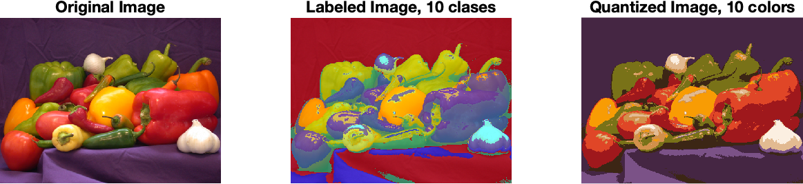
Fig. 1 Example of segmentation using the K-means clustering function at K=10, on the right is the original image, in the center the 10 resulting clusters are shown, on the right is an example of the use of clusters and their centroids for image quantization
References
[1] Gonzalez, R., C., Woods, E., W., Digital Image Processing, Global Edition, 4th edition, Pearson 2018, ISBN 10: 1-292-22304-9
Appendix
The source code of the program that created Fig. 1
clear all; close all; clc;
clnum=10;
fig=figure;
subplot(1,3,1)
I = imread("peppers.png");
imshow(I)
title("Original Image")

subplot(1,3,2)
[L,Centers] = imsegkmeans(I,clnum);
B = labeloverlay(I,L);
imshow(B)
title("Labeled Image, 10 clases")

subplot(1,3,3)
[L,Centers] = imsegkmeans(I,clnum);
J = label2rgb(L,im2double(Centers));
imshow(J)
title("Quantized Image, 10 colors")
fig.PaperUnits = 'inches';
fig.PaperPosition = [0 0 10 6];
print(fig,"segmColorKmeans.png",'-dpng');
The PDF version of this text is available here: segmentation_color_kmeans_eng.pdf