Local thresholding
Global thresholding does not consider the position of the points. There are several ways to take the position of the points into account and improve the quality of the segmentation using thresholding.
The first way is to use image smoothing. For example, when we have a noisy image, smoothing will help to suppress the noise and recover the maxima in the histogram of the image. It is important to remember that if we are smoothing e.g. averaging using filter with a kernel of 5x5 points, so we actually use the local neighborhood of 5x5 points. On the other hand, smoothing can cause deformation of the edges of the object, so a compromise must be sought between the force of smoothing and the deformation caused. An example of a successful improvement of global thresholding by image smoothing is shown in Fig. 1.
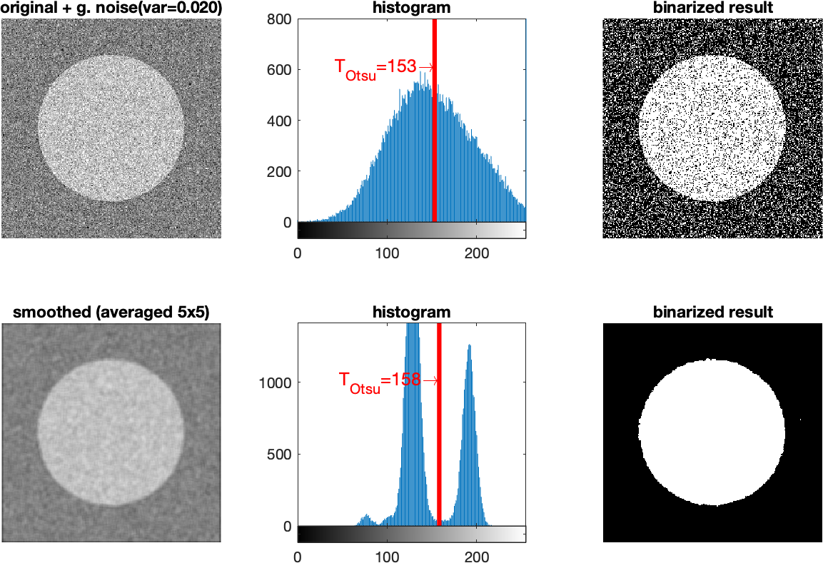
Fig. 1 Example of successful improvement of Otsu thresholding by smoothing (In the upper row of images, the original noisy image is on the left, its histogram in the middle, and unsuccessful Otsu thresholding on the right. In the lower row, the original noisy image smoothed with a 5x5 averaging filter is on the left, its histogram in the middle, and successful Otsu thresholding on the right )
If the object in the foreground contains few points compared to the points in the background (i.e. its contribution is negligible within the histogram), then smoothing may not help (or it may do more harm). It can be a significant help to use a mask when calculating the histogram and take into account only values from a reasonably large area around the object. We can get the mask manually or (semi)automatically. Alternatively, we will take into account only the points around the edge between the object and the background (e.g. the Laplacian can provide us such a mask).
Noise in the image, a small object in the foreground are just two of the many situations where it would help to consider the surroundings when performing thresholding. Fig. 2 shows a situation with shadows in the form of stripes across the entire image, where it is desirable to use a thresholding method that takes into account the local characteristics of the image. Most often, the mean and variance are taken into account as local characteristics [1]. In the MATLAB environment, there is a function adaptthresh that selects the threshold adaptively based on the local average (mean). An example of the use of this function for local thresholding of an image with unequal background illumination is given on Fig. 3. We can see that in the lower part the global Otsu thresholding fails, while the local one succeeds in maintaining the standard quality.
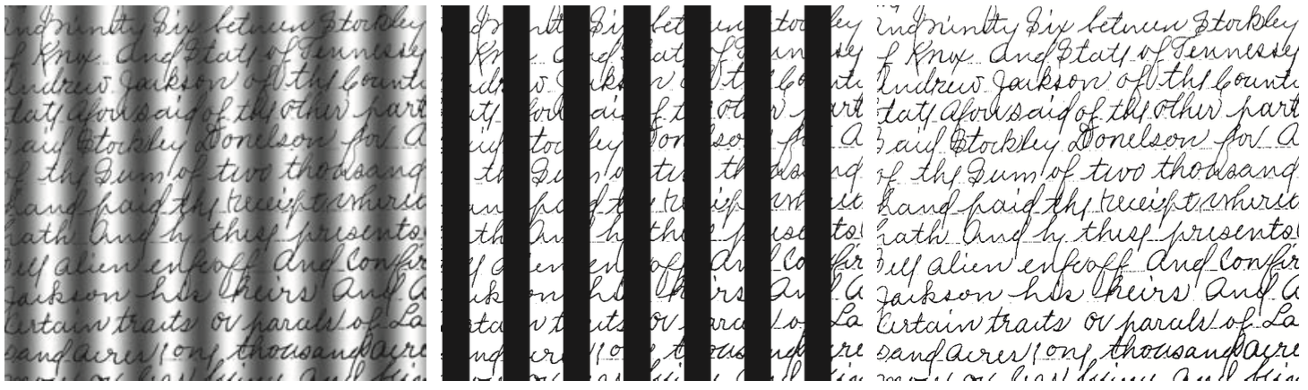
Fig. 2 The advantage of local approach when thresholding. On the left is the original image, in the middle is global Otsu thresholding, on the right is thresholding using the local average [1]
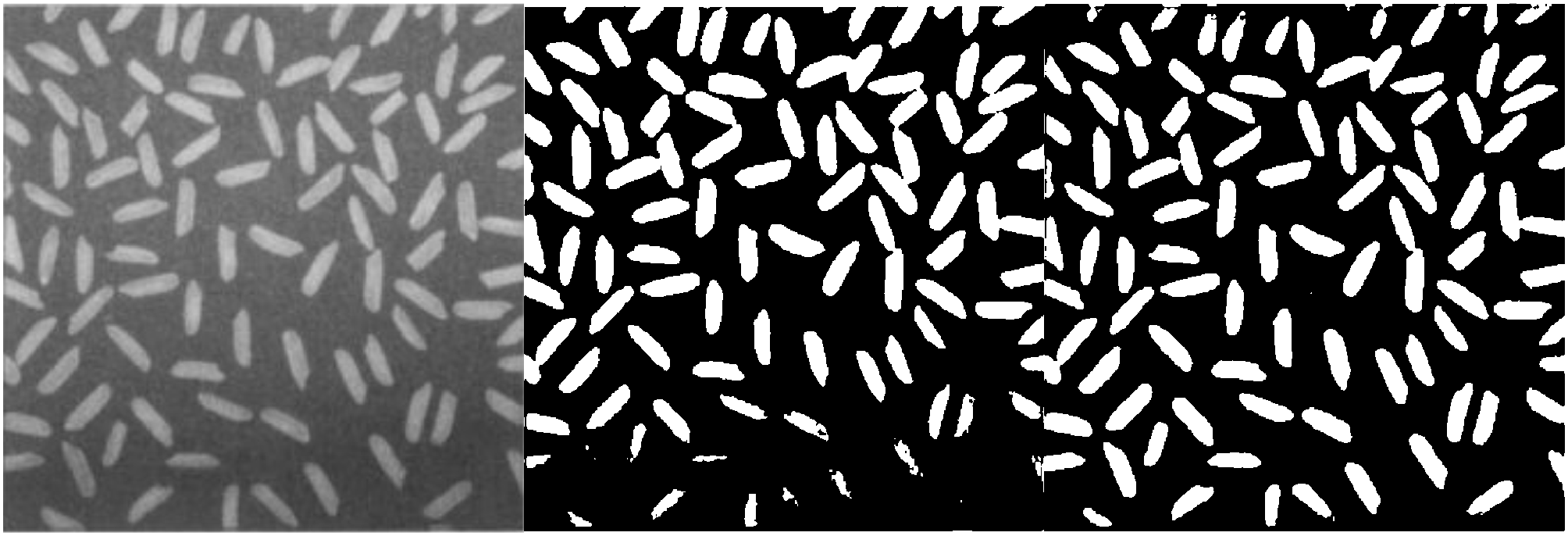
Fig. 3 Comparison of global and local thresholding on the example of image with uneven brightness. Original on the left, Otsu thresholding in the middle, thresholding using the local average on the right
References
[1] Gonzalez, R., C., Woods, E., W., Digital Image Processing, Global Edition, 4th edition, Pearson 2018, ISBN 10: 1-292-22304-9
Appendix
The source code of the program that created Fig. 1
clear all; close all; clc;
N=256
mtx=uint8(128*ones(N,N));
imshow(mtx,[0,255]);
h = drawcircle('Center',[N/2 N/2],"Radius",N/3);
mask = createMask(h);
mtx(mask>0)=128+64;

fig=figure
subplot(2,3,1)
myvar=0.02
mtxn = imnoise(mtx,'gaussian',0,myvar);
imshow(mtxn,[0,255]);
title(sprintf("original + g. noise(var=%.3f)",myvar))

subplot(2,3,2)
imhist(mtxn);
hold on
[T,EM] = graythresh(mtxn)
myT=T*255;
myYlim=ylim;
plot([myT myT],[myYlim(1) myYlim(2)],"red","LineWidth",3)
text(myT,600,sprintf("T_{Otsu}=%.0d\\rightarrow",myT),...
    'HorizontalAlignment','right',"FontSize",12,"Color","red")
title("histogram")


subplot(2,3,3)
BW = imbinarize(mtxn,T);
imshow(BW);
title("binarized result")

subplot(2,3,4)
myFilt=1/25*ones(5,5)
mtxn = imfilter(mtxn,myFilt);
imshow(mtxn,[0,255]);
title(sprintf("smoothed (averaged 5x5)",myvar))

subplot(2,3,5)
imhist(mtxn);
hold on
[T,EM] = graythresh(mtxn)
myT=T*255;
myYlim=ylim;
plot([myT myT],[myYlim(1) myYlim(2)],"red","LineWidth",3)
text(myT,1000,sprintf("T_{Otsu}=%i\\rightarrow",myT),...
    'HorizontalAlignment','right',"FontSize",12,"Color","red")
title("histogram")


subplot(2,3,6)
BW = imbinarize(mtxn,T);
imshow(BW);
title("binarized result")

fig.PaperUnits = 'inches';
fig.PaperPosition = [0 0 10 6];
print(fig,"segmOtsuSmooth.png",'-dpng');
The source code of the program that created Fig. 3
clear all; close all; clc;
I = im2gray(imread('rice.png'));
Totsu = graythresh(I)
BWotsu = imbinarize(I,Totsu);
Tadapt = adaptthresh(I, 0.5);
BWadapt = imbinarize(I,Tadapt);
montage({I,BWotsu,BWadapt},"Size",[1,3]);
exportgraphics(gcf(),'segmLocalAdapt.png')
The PDF version of this text is available here: segmentation_local_tresholding_eng.pdf