DIP: Optimal global thresholding

A well-known and effective method for global thresholding is the Otsu method [1]. It is optimal in the sense that it maximizes the variance $\sigma_B^2$ between classes. The algorithm is not iterative, but usually all threshold values are checked for optimality. We are looking for which threshold value $T$ is $\sigma_B^2(T)$ maximum:

$\sigma_B^2(T) = P_1(T)\left( m_1(T) - m_G\right) ) ^2 + P_2(T)\left( m_2(T) - m_G\right) ) ^2$

where

$m_G =\sum_{i=0}^{L-1} i p_i$

$m_1 (T)=\frac{1}{P_1 (T)}\sum_{i=0}^T i p_i$

$m_2 (T)=\frac{1}{P_2 (T)}\sum_{i=T+1}^{L-1} i p_i$

where

$P_1(T)=\sum_{i=0}^T p_i$

$P_2(T)=\sum_{i=T+1}^{L-1} p_i$

$p_i=\frac{n_i}{M N}$

where $n_i$ is the number of points with brightness level $i$ , $L$ is the number of brightness levels in the image $M, N$ are the dimensions of the image. It turns out that the maximum always exists. If the maximum is reached for several $T$ values, the average of these values is usually considered as the result.

The derivation of the mentioned algorithm and the discussion of its properties is given in [1].

Analogously, it is possible to derive a relation for $K$ classes for which we are looking for $K-1$ optimal thresholds $T_1, ..T_{K-1}$ . Then we maximize:

$\sigma_B^2 = \sum_{j=1}^{K} P_j\left( m_j - m_G\right) ) ^2$

where

$m_j=\frac{1}{P_j}\sum_{i=T_{j-1}+1}^{T_j} i p_i$

$P_j=\sum_{i=T_{j-1}+1}^{T_j} p_i$

$p_i=\frac{n_i}{M N}$

where $n_i$ is the number of points with brightness level $i$ , $L$ is the number of brightness levels in the image, $M, N$ are the dimensions of the image and $T_0=-1, T_K= L-1$

In the MATLAB environment, Otsu thresholding is implemented using the function graythresh (argument is an image) and otsuthresh (argument is the number of points $n_i$ with brightness level $i$ ) - for two classes and multithresh - for multiple classes.

An example of the use of Otsu thresholding is shown in Fig. 1. The task is to find the optimal threshold between two classes. We see how the presence of stronger noise can make it difficult to determine the threshold.

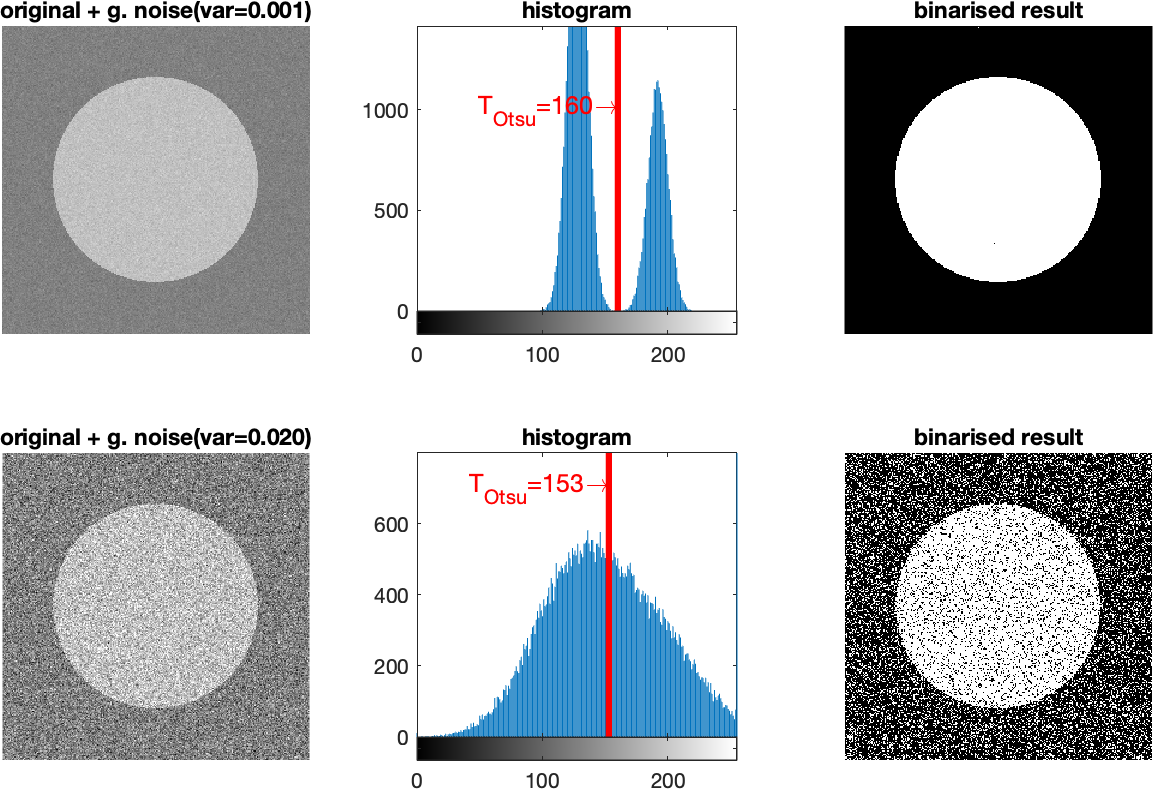
Fig. 1 Example of Otsu thresholding with a noisy input signal. In the upper row there is a weaker noisy signal, in the lower

Fig. 1 Example of Otsu thresholding with a noisy input signal. In the upper row there is a weaker noisy signal, in the lower row it is stronger

References

[1] Gonzalez, R., C., Woods, E., W., Digital Image Processing, Global Edition, 4th edition, Pearson 2018, ISBN 10: 1-292-22304-9

Appendix

The source code of the program that created Fig. 1

clear all; close all; clc;
N=256
mtx=uint8(128*ones(N,N));
imshow(mtx,[0,255]);
h = drawcircle('Center',[N/2 N/2],"Radius",N/3);
mask = createMask(h);
mtx(mask>0)=128+64;

fig=figure
subplot(2,3,1)
myvar=0.001
mtxn = imnoise(mtx,'gaussian',0,myvar);
imshow(mtxn,[0,255]);
title(sprintf("original + g. noise(var=%.3f)",myvar))

subplot(2,3,2)
imhist(mtxn);
hold on
[T,EM] = graythresh(mtxn)
myT=T*255;
myYlim=ylim;
plot([myT myT],[myYlim(1) myYlim(2)],"red","LineWidth",3)
text(myT,1000,sprintf("T_{Otsu}=%.0d\\rightarrow",myT),...
    'HorizontalAlignment','right',"FontSize",12,"Color","red")
title("histogram")


subplot(2,3,3)
BW = imbinarize(mtxn,T);
imshow(BW);
title("binarised result")

subplot(2,3,4)
myvar=0.2
mtxn = imnoise(mtx,'gaussian',0,myvar);
imshow(mtxn,[0,255]);
title(sprintf("original + g. noise(var=%.3f)",myvar))

subplot(2,3,5)
imhist(mtxn);
hold on
[T,EM] = graythresh(mtxn)
myT=T*255;
myYlim=ylim;
plot([myT myT],[myYlim(1) myYlim(2)],"red","LineWidth",3)
text(myT,700,sprintf("T_{Otsu}=%i\\rightarrow",myT),...
    'HorizontalAlignment','right',"FontSize",12,"Color","red")
title("histogram")


subplot(2,3,6)
BW = imbinarize(mtxn,T);
imshow(BW);
title("binarised result")

fig.PaperUnits = 'inches';
fig.PaperPosition = [0 0 10 6];
print(fig,"segmOtsuNoise.png",'-dpng');

The PDF version of this text is available here: segmentation_otsu_eng.pdf