Image stitching
When capturing an image, sometimes our capture device cannot cover the entire scene. One of the solutions is to capture parts of the scene and then put those parts together in such way that is not visible that the resulting image is composition. This process is called image stitching. In this process we create the resulting image from the tiles of individual partial images. These tiles must "fit" each other and the place where they were sewn together should not be visible. This task is not trivial considering that we do not shoot from the same point at the same time and we often are not able to manage that the borders of the images match so the images smoothly do not connect to each other. The geometric imperfections of the sensor and other circumstances are further complications. If we know that we are going to stitch the resulting scene, then when shooting partial parts, it is appropriate:
- shoot under the same external conditions, so that the scene changes minimally (position of objects, lighting), i.e. usually as quickly as possible
- shoot under the same internal conditions, i.e. sensor parameters (disable automatic settings of sensing parameters, auto-focus, do not change the settings, ...)
- to have an overlap of partial parts of at least 20-30\% so that there is sufficient overlap for stitching
We can look at image stitching as creating a panorama (an image of the observer's surroundings). The two basic types of panorama are rotational and translational. If the observer does not move from his place (only turns and looks around), we speak of a rotational panorama. If he does not turn, but moves and always looks in one direction (e.g. through the window of a car driving down the street), we speak of a translational panorama. The rotating panorama can be considered a simpler problem, because it composes the surroundings as it looks from one point, which has a unambiguous solution (in an idealized case). When the observation point moves, the observed area can look different from different observation points - different reflections, different shape (we are usually looking at a three-dimensional area). If we observe only the area perpendicular to the direction of movement (such as scanners do), then the image is unambiguous, but we need many images. The image is unambiguous also even if the scene is flat and without glare. The basic situation when capturing source images for translational and rotational panoramas is shown in Fig. 1.
![]()
Fig. 1 Schematic picture of scanning when creating a translational (left) and rotational (right) panorama.
In the case of a rotating panorama, if the objects are not at the same distance from the observer, we see the effect of perspective in the side views - initially parallel edges of the building point later towards each other. This must be taken into account when stitching. An example of stitching with a rotating panorama, where we try to preserve the geometry of the central image, is shown in Fig. 2. We see that if we choose (correctly) the third image in the sequence as the central one, and stitch the surrounding images to it, then we have to stretch the outer images more and more vertically. The resulting image has the shape of butterfly wings. And if we choose the wrong image as the central image, then when correcting the influence of perspective, the entire image will be slanted.
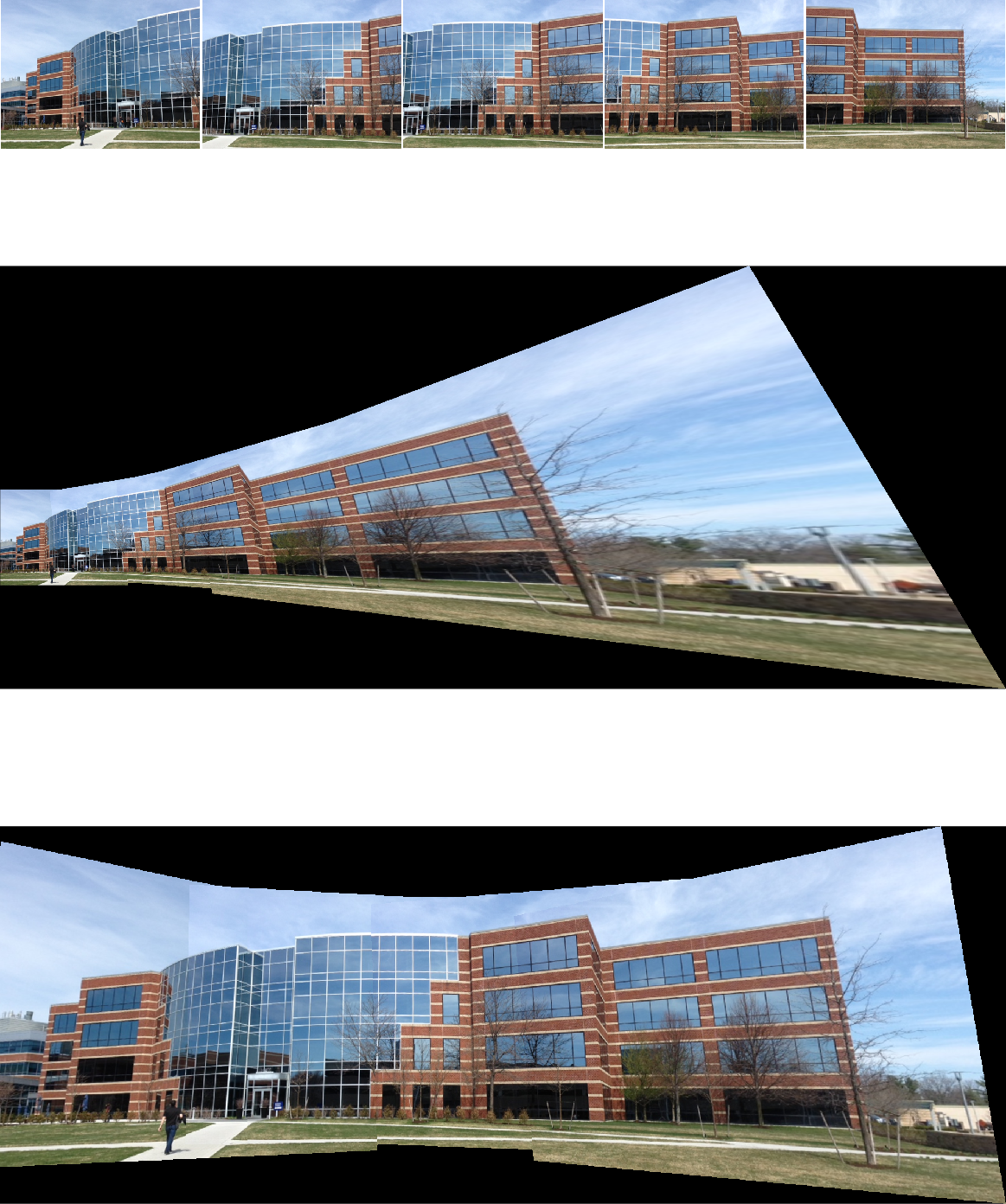
Fig. 2 Example of stitching a rotating panorama. The sequence of images taken is in the upper part, in the middle is shown the stitched panorama when the left image was selected as the central image, in the bottom part is shown the stitched panorama when the middle image was selected as the central image. When stitching, SURF was used to detect key points, MSAC to find the projective transform, and simplest pixel based binary blending was used.
The stitching algorithm has to solve several problems:
- Choose the target projection (flat cylindrical, spherical) - on which surface we will construct the result.
- Find out how the images overlap. De facto image registration is performed - mapping of images into a common coordinate system. As a rule, one image is chosen as the central one, and the transformation of the surrounding images is sought for it, so that they overlap as best as possible.
- Determining the border between stitched images - where the seam will go. A trivial choice is around the edge of the image, but more sophisticated methods look for where the images match as much as possible and lead the seam there. Alternatively, it is sewn along the edges, where the seam is well visually disguised.
- Choice of blending method - a trivial and intuitive method is to use pixels of one image on one side of the seam and pixels of the other image on the other side of the seam. Alternatively, the values around the seam can be averaged or weighted, blending based on translucency (alpha blending) or blending using Laplace pyramids can be used, or the blending as when creating an image with a high dynamic range can be used.
Details of how the stitching of the image was gradually carried out in the lower part of Fig. 2 are shown in Fig. 3
The stitching algorithm has to address several problems:
- Choose the target projection (flat cylindrical, spherical) - on which surface we will construct the result.
- Find out how the images overlap. De facto image registration is performed - mapping of images into a common coordinate system. As a rule, one is chosen as the central one, and the transformation of the surrounding images is sought for it, so that they overlap as best as possible.
- Determining the border between stitched images - where the seam will go. A trivial choice is around the edge of the image, but more sophisticated methods look for where the images match as much as possible and lead the seam there. Alternatively, it is sewn along the edges, where the seam is well visually disguised.
- Choice of blending method - a trivial and intuitive method is to use pixels of one image on one side of the seam and pixels of the other image on the other side of the seam. Alternatively, the values around the seam can be averaged or weighted, blending based on translucency (alpha blending) or blending using Laplace pyramids can be used, or the principle of blending can be used as when creating an image with a high dynamic range.
Details of how the stitching of the image was gradually carried out in the lower part of Fig. 2 are shown in Fig. 3
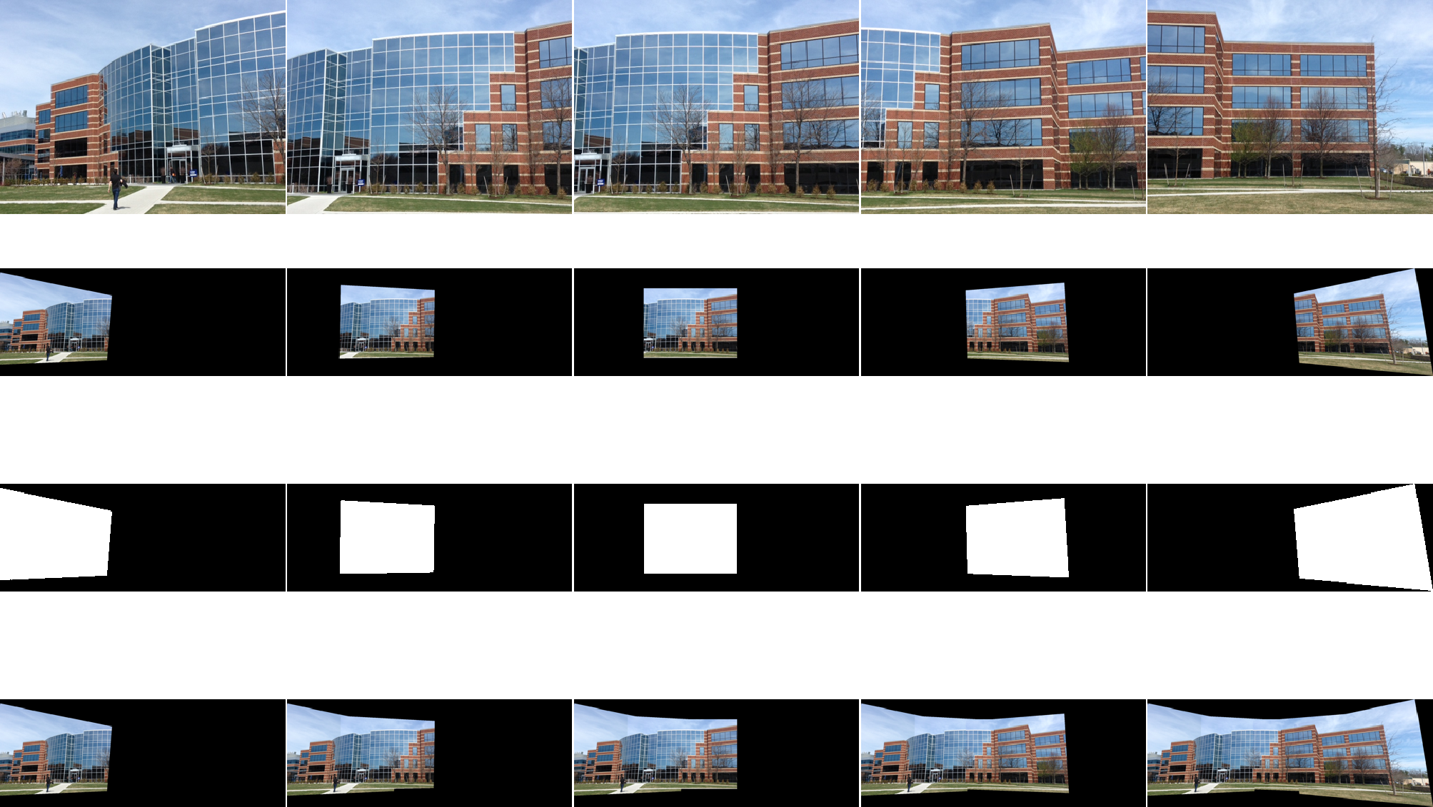
Fig. 3 An example of the detail in the stitching process; in the top row we see the originals; below them their registered versions; below them a binary mask that determines which of their pixels will be used (we can see that all pixels will be used, that is, the seam is placed along their left edge; at the bottom the state of the overall panoramas after stitching the image in the given step)
When stitching as displayed on Fig. 2, the specific stitching algorithm was used as follows [1]:
- Select power projection: flat surface
- Label images as \(I(1), ...I(5)\)
- For each image pair \(I(n), ...I(n-1)\) perform registration, find the transformation \(I(n)\) to the coordinate system \(I(n-1)\)
- Using the SURF method identify the salient points on both \(I(n)\) and \(I(n-1)\) . MATLAB: detectSURFFeatures() + extractFeatures()
- Search among them for unique pairs with the best match (MATLAB: matchFeatures(), with the option "Unique") based on the SAD (Sum of Absolute Differences) metric
- Based on pairs of points, estimate the transformation \(I(n)\) into the coordinate system of \(I(n-1)\) using the MSAC (M-estimator sample consensus) method, which is a variant of the well-known RANSAC (random sample consensus) method , looking for the projective transformation (MATLAB: estgeotform2d() with the parameter "projective" )
- calculate the resulting transformation \(I(n)\) against the initial \(I(1)\) as \(\prod_{n=1}^n T(n)\)
- If the central image is different from \(I(1)\) recalculate\(T(n)\) against this image
- To \(I(1)\) gradually sew other images, using the transformed edge of the stitched image as a seam and using the simplest blending, i.e. add exactly the full pixel values in the area of the new image (MATLAB: vision.AlphaBlender, while the operation is "Binary mask")
Unlike the situation in Fig. 2, where the stitching took place horizontally, in real panoramas it is often stitched in the other direction as well, i.e. the resulting image is formed e.g. from 20x10 input overlapping images. There are a number of specialized programs for image stitching (an excellent review can be found, for example, in [2])
References
[1] Mathworks, Feature Based Panoramic Image Stitching, http://www.mathworks.com/help/vision/ug/feature-based-panoramic-image-stitching.html
[2] Comparison of photo stitching software, wikipedia, https://en.wikipedia.org/wiki/Comparison_of_photo_stitching_software#:~:text=Photo%20stitching%20software%20produce%20panoramic,more%20or%20less%20smooth%20image.
Appendix
The source code of the program that created Fig. 2 and Fig.3
  clear all;close all;clc;
%https://www.mathworks.com/help/vision/ug/feature-based-panoramic-image-stitching.html
% Load images.
buildingDir = fullfile(toolboxdir('vision'),'visiondata','building');
buildingScene = imageDatastore(buildingDir);

[tforms,imageSize]=getTformsSizes(buildingScene);
panorama0=getPanorama(buildingScene,tforms,imageSize,0);
panorama1=getPanorama(buildingScene,tforms,imageSize,1);

fig=figure;
subplot(5,1,[1 1]);
montage(buildingScene.Files,"Size",[1 5], "BorderSize", [2 2],"BackgroundColor","w");
subplot(5,1,[2 3]);
imshow(panorama0)
subplot(5,1,[4 5]);
imshow(panorama1)
fig.PaperUnits = 'inches';
fig.PaperPosition = [0 0 10 12];
print(fig,"stitching.png",'-dpng');


%=========================================================
function [tforms,imageSize]=getTformsSizes(buildingScene)

    % Read the first image from the image set.
    I = readimage(buildingScene,1);

    % Initialize features for I(1)
    grayImage = im2gray(I);
    points = detectSURFFeatures(grayImage);
    [features, points] = extractFeatures(grayImage,points);

    % Initialize all the transformations to the identity matrix. Note that the
    % projective transformation is used here because the building images are fairly
    % close to the camera. For scenes captured from a further distance, you can use
    % affine transformations.
    numImages = numel(buildingScene.Files);
    tforms(numImages) = projtform2d;

    % Initialize variable to hold image sizes.
    imageSize = zeros(numImages,2);

    % Iterate over remaining image pairs
    for n = 2:numImages
        % Store points and features for I(n-1).
        pointsPrevious = points;
        featuresPrevious = features;
        % Read I(n).
        I = readimage(buildingScene, n);
        % Convert image to grayscale.
        grayImage = im2gray(I);
        % Save image size.
        imageSize(n,:) = size(grayImage);
        % Detect and extract SURF features for I(n).
        points = detectSURFFeatures(grayImage);
        [features, points] = extractFeatures(grayImage, points);
        % Find correspondences between I(n) and I(n-1).
        indexPairs = matchFeatures(features, featuresPrevious, 'Unique', true);
        matchedPoints = points(indexPairs(:,1), :);
        matchedPointsPrev = pointsPrevious(indexPairs(:,2), :);
        % Estimate the transformation between I(n) and I(n-1).
        tforms(n) = estgeotform2d(matchedPoints, matchedPointsPrev,...
            'projective', 'Confidence', 99.9, 'MaxNumTrials', 2000);
        % Compute T(1) * T(2) * ... * T(n-1) * T(n).
        tforms(n).A = tforms(n-1).A * tforms(n).A;
    end
end

%=========================================================
function panorama = getPanorama(buildingScene,tforms,imageSize,doCentering)

    if(doCentering)
        % Compute the output limits for each transformation.
        for i = 1:numel(tforms)
            [xlim(i,:), ylim(i,:)] = outputLimits(tforms(i), [1 imageSize(i,2)], [1 imageSize(i,1)]);
        end

        avgXLim = mean(xlim, 2);
        [~,idx] = sort(avgXLim);
        centerIdx = floor((numel(tforms)+1)/2);
        centerImageIdx = idx(centerIdx);

        Tinv = invert(tforms(centerImageIdx));
        for i = 1:numel(tforms)
            tforms(i).A = Tinv.A * tforms(i).A;
        end
    end

    for i = 1:numel(tforms)
        [xlim(i,:), ylim(i,:)] = outputLimits(tforms(i), [1 imageSize(i,2)], [1 imageSize(i,1)]);
    end

    maxImageSize = max(imageSize);

    % Find the minimum and maximum output limits.
    xMin = min([1; xlim(:)]);
    xMax = max([maxImageSize(2); xlim(:)]);
    yMin = min([1; ylim(:)]);
    yMax = max([maxImageSize(1); ylim(:)]);
    % Width and height of panorama.
    width  = round(xMax - xMin);
    height = round(yMax - yMin);
    % Initialize the "empty" panorama.
    I = readimage(buildingScene,1);
    panorama = zeros([height width 3], 'like', I);
    blender = vision.AlphaBlender('Operation', 'Binary mask', ...
        'MaskSource', 'Input port');
    % Create a 2-D spatial reference object defining the size of the panorama.
    xLimits = [xMin xMax];
    yLimits = [yMin yMax];
    panoramaView = imref2d([height width], xLimits, yLimits);
    numImages = numel(buildingScene.Files);
    % Create the panorama.
    for i = 1:numImages;

        I = readimage(buildingScene, i);
        imwrite(I,sprintf("img%02i.png",0*5+i));
        % Transform I into the panorama.
        warpedImage = imwarp(I, tforms(i), 'OutputView', panoramaView);
        imwrite(warpedImage,sprintf("img%02i.png",1*5+i));
        % Generate a binary mask.
        mask = imwarp(true(size(I,1),size(I,2)), tforms(i), 'OutputView', panoramaView);
        imwrite(mask,sprintf("img%02i.png",2*5+i));
        % Overlay the warpedImage onto the panorama.
        panorama = step(blender, panorama, warpedImage, mask);
        imwrite(panorama,sprintf("img%02i.png",3*5+i));
    end
    fig=figure
    imds = imageDatastore(fullfile(".","img*"));
    montage(imds,"Size", [4 5],"BorderSize", [1 1],"BackgroundColor","w")
    print(fig,sprintf("stitchingDetailsDC%u.png",doCentering),'-dpng');
end
The PDF version of this text is available here: stitching_eng.pdf