Grayscale morphology
In addition to a black and white image morphology, the morphology is also very useful in grayscale image processing. All 4 basic operations erosion, dilation, opening, closing are used. Using grayscale morphology, we have a choice whether we want to use a flat (with a constant intensity value) structural element or a non-flat one.
Let \(f(x,y)\) be an image and \(b(x,y)\) a structural element. Then erosion \(f(x,y)\) using \(b(x,y)\) is defined as
- for a flat structural element are the new image values minimum from the surroundings of the given element
\[ \left[ f\ominus b\right] (x,y)=\min_{(s,t)\in b} \left\lbrace f(x+s, y+t) \right\rbrace \]
- for a non-flat structural element \(b_N\), the value of the element is also taken into account
\[ \left[ f\ominus b_N\right] (x,y)=\min_{(s,t)\in b} \left\lbrace f(x+s, y+t) -b_N(s,t ) \right\rbrace \]
Similarly, dilation is defined as
- for a flat structural element, the new image values are maximums from the rotated neighborhood of the given element
\[ \left[ f\ominus b\right] (x,y)=\max_{(s,t)\in b} \left\lbrace f(x-s, y-t) \right\rbrace \]
- for a non-flat structural element \(b_N\), the value of the element is also taken into account
\[ \left[ f\ominus b_N\right] (x,y)=\max_{(s,t)\in b} \left\lbrace f(x-s, y-t) -\widehat{b_N}(s,t ) \right\rbrace \]
Opening and closing are defined by dilation and erosion just as it is in a black and white image. In the MATLAB environment, these are the same functions: imdilate, iimerode, imopen, imclose. Examples of all mentioned operations are shown in Fig. 1.
Another operation is morphological smoothing. It is a combination of opening and then closing. An example of this operation is shown in Fig. 2.
An interesting operation is morphological gradient (MG), in which the eroded image is subtracted from the dilated image (which should highlight the boundaries of the objects):
\[I_{MG}=(A\oplus B)- (A\ominus B)\]
An example of this operation is shown in Fig. 3.
Grayscale morphology can also be used as preprocessing before segmentation. For example the top-hat operation is used to equalize scene illumination before global segmentation:
\[I_{TH}= I - (I \circ B)\]
An example of this operation is shown in Fig. 4.
The top-hat operation can also be used for blob detection. It exploits the property, that if the size of the blob and the structural element are similar, the blobs in the image become darker when the opening is subtracted from the image. So we can construct a brightness after the toop-hat operation as a function of Structural Element size. It is better to display the first derivative (gradient) of this function. There, you just need to look for the maximum value and, based on that, determine whether there are blobs in the image and what their size is. An example of such use of top-hat is shown in Fig. 5. If we work with the unsmoothed version of the image (above), then the maximum change in brightness is due to noise at small values of the size of the structural element. On the smoothed version of the image, we see the maximum values of the gradients of changes in the brightness of the openings at the sizes of the structural element 19 and 27.
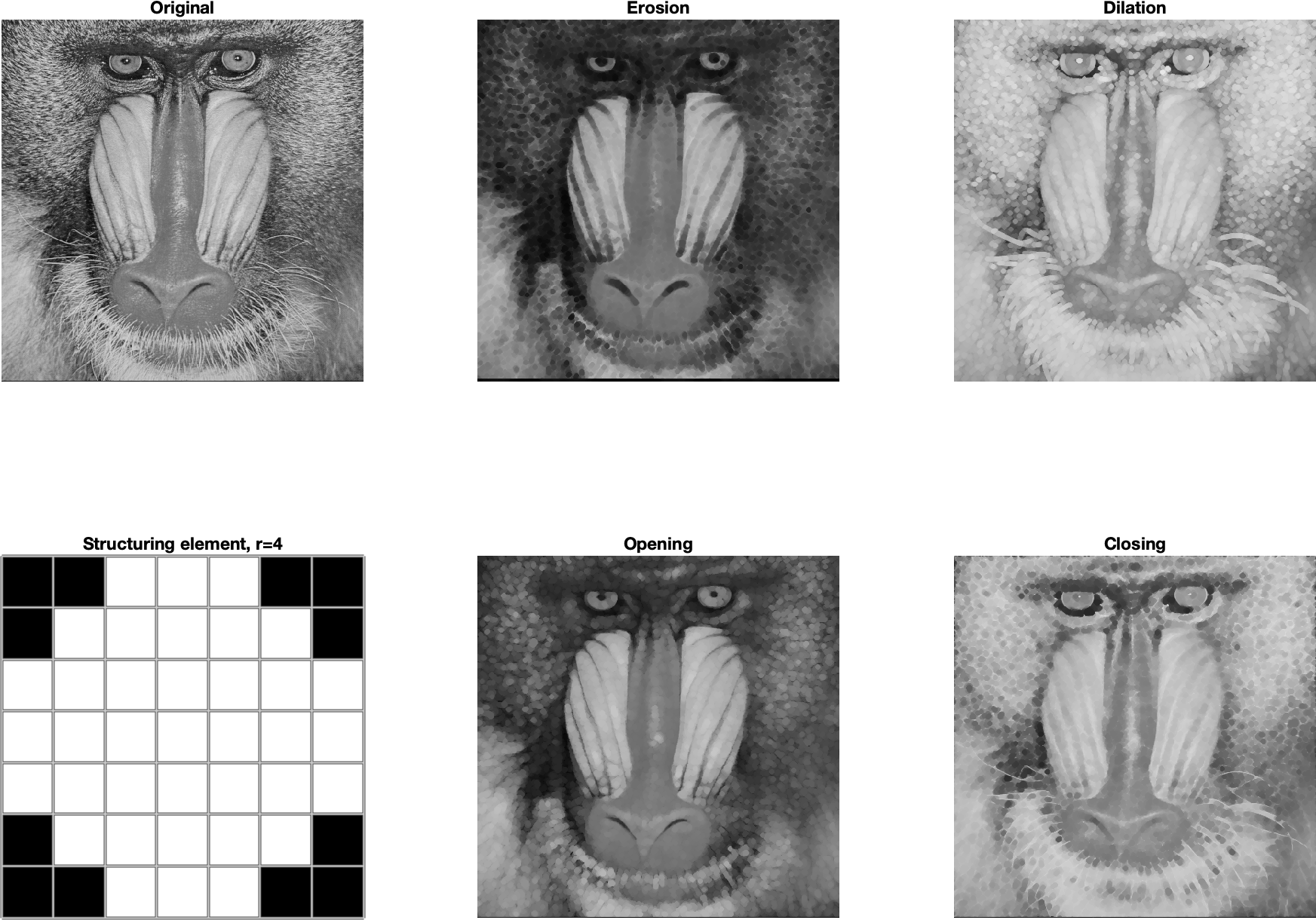
Fig. 1 Examples of basic morphological operations erosion, dilation, opening, closing for grayscale image.
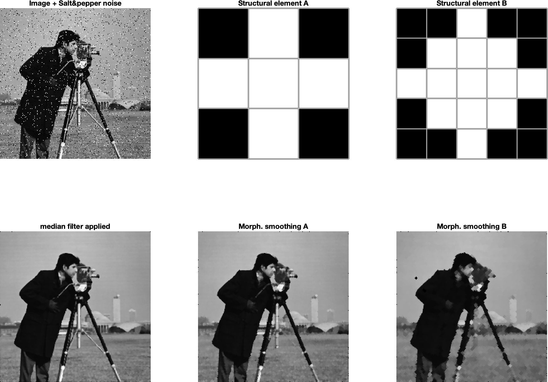
Fig. 2 Examples of morphological smoothing and comparison with the median filter.
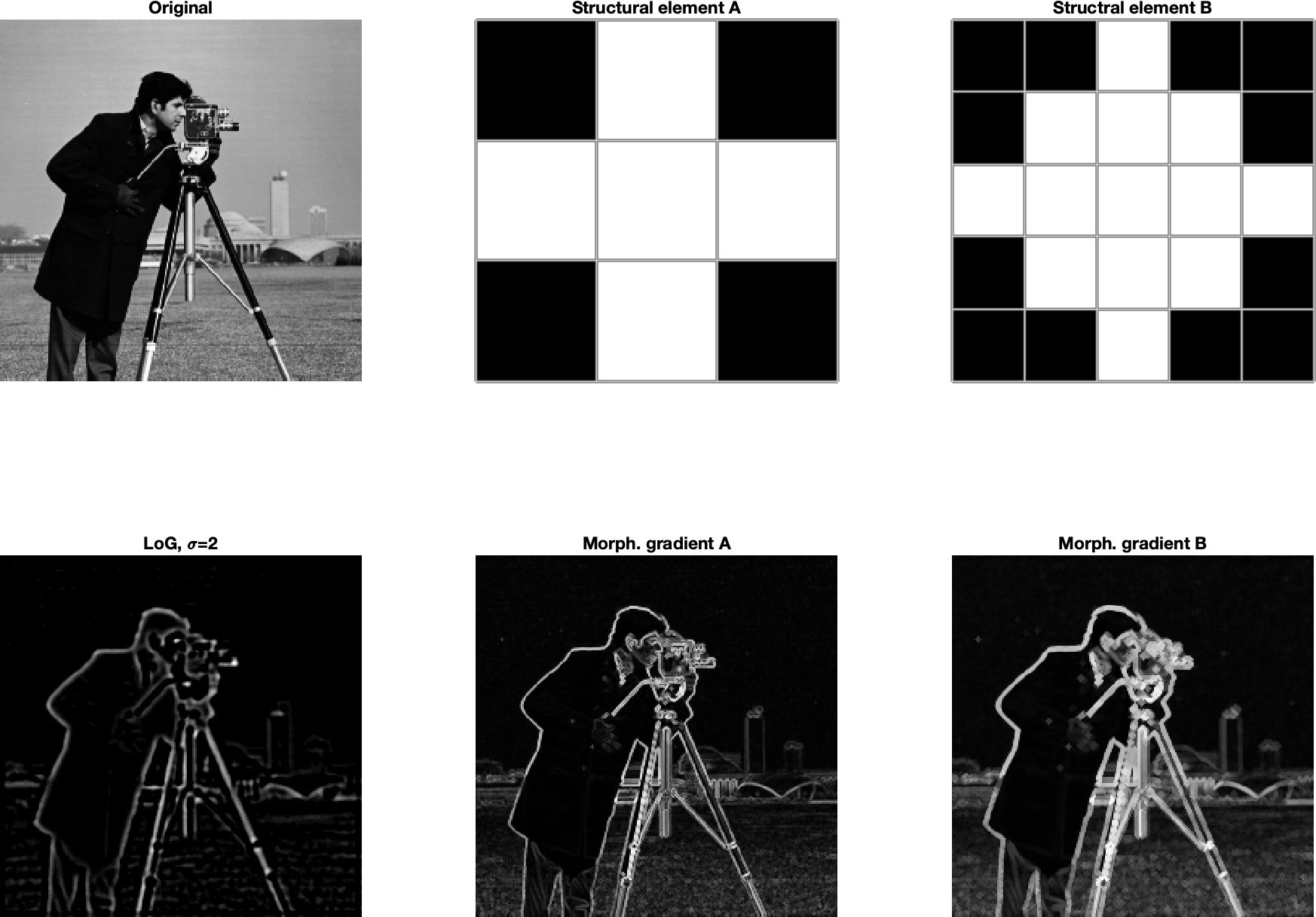
Fig. 3 Examples of morphological gradient and comparison with LoG filter.
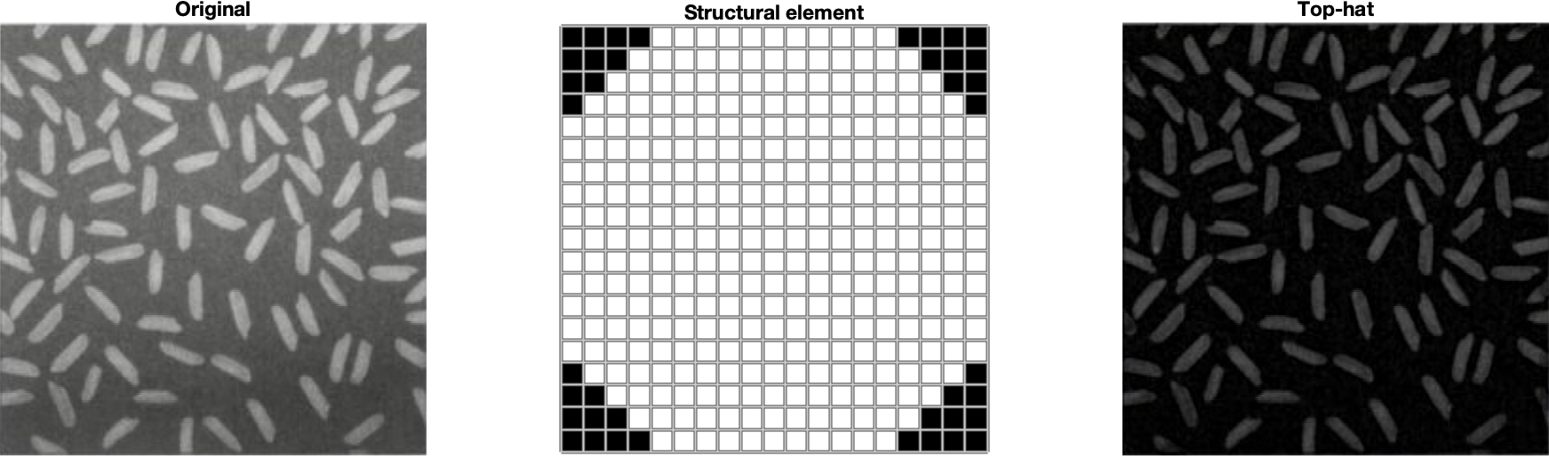
Fig. 4 Example of using the top-hat operation to equalize scene lighting
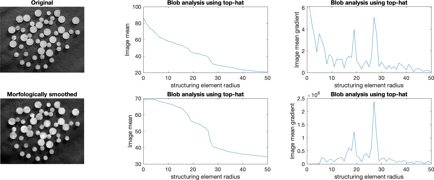
Fig. 5 Example of using repeated top-hat operation for blob detection.
References
[1] Mathworks, Morphological Operations, online: https://www.mathworks.com/help/images/morphological-filtering.html
[2] Gonzalez, R., C., Woods, E., W., Digital Image Processing, Global Edition, 4th edition, Pearson 2018, ISBN 10: 1-292-22304-9
[3] Gonzalez, R., C., Woods, E., W., Eddings, S., L., Digital Image Processing using MATLAB, Gatesmark Publishing, ISBN-10: 0-9820854-1-9
Appendix
The source code of the program that created Fig. 1
clear all; close all; clc;
fig=figure;
A=im2gray(imread('baboon.png'));
subplot(2,3,1)
showCol(A,'Original');

subplot(2,3,4)
B=strel('disk',4);
showCol(B.Neighborhood,'Structuring element, r=4')
pixelgrid;

subplot(2,3,2)
C=imerode(A,B);
showCol(C,'Erosion')

subplot(2,3,3)
C=imdilate(A,B);
showCol(C,'Dilation')

subplot(2,3,5)
C=imopen(A,B);
showCol(C,'Opening')

subplot(2,3,6)
C=imclose(A,B);
showCol(C,'Closing')

fig.PaperUnits = 'inches';
fig.PaperPosition = [0 0 15 10];
print(fig,'morphGrayBasicOps.png','-dpng');

function showCol(myImg, myTitle)
    imshow(myImg);
    title(myTitle)
end
The source code of the program that created Fig. 2
clear all; close all; clc;
fig=figure;
ORIG= imread('cameraman.tif');
SP = imnoise(ORIG,'salt & pepper');
subplot(2,3,1);
imShowTit(SP,"Image + Salt&pepper noise")
subplot(2,3,4);
MF=medfilt2(SP);
imShowTit(MF, "median filter applied")
subplot(2,3,2);
SE = strel("disk",1);
imShowTit(double(SE.Neighborhood), "Structural element A")
pixelgrid;
subplot(2,3,5);
OP=imopen(SP,SE);
CL=imclose(OP,SE);
imShowTit(CL, "Morph. smoothing A")
subplot(2,3,3);
SE = strel("disk",2);
imShowTit(double(SE.Neighborhood), "Structural element B")
pixelgrid;
subplot(2,3,6);
OP=imopen(SP,SE);
CL=imclose(OP,SE);
imShowTit(CL, "Morph. smoothing B")

fig.PaperUnits = 'inches';
fig.PaperPosition = [0 0 15 10];
print(fig,'morphGrayBasicSmooth.png','-dpng');

function imShowTit(myImg, myTitle)
    imshow(myImg);
    title(myTitle)
end
The source code of the program that created Fig. 3
clear all; close all; clc;
fig=figure;
SP= imread('cameraman.tif');
subplot(2,3,1);
imShowTit(SP,'Original')
subplot(2,3,4);
myFilt = fspecial('log',10,2);
myLog=imfilter(SP,myFilt);
imShowTit(myLog,'LoG, \sigma=2')
subplot(2,3,2);
SE = strel('disk',1);
imShowTit(double(SE.Neighborhood), 'Structural element A')
pixelgrid;
subplot(2,3,5);
CL=imdilate(SP,SE)-imerode(SP,SE);
imShowTit(CL, 'Morph. gradient A')
subplot(2,3,3);
SE = strel('disk',2);
imShowTit(double(SE.Neighborhood), 'Structral element B')
pixelgrid;
subplot(2,3,6);
CL=imdilate(SP,SE)-imerode(SP,SE);
imShowTit(CL, 'Morph. gradient B')

fig.PaperUnits = 'inches';
fig.PaperPosition = [0 0 15 10];
print(fig,'morphGrayBasicGrad.png','-dpng');

function imShowTit(myImg, myTitle)
    imshow(myImg,[]);
    title(myTitle)
end
The source code of the program that created Fig. 4
clear all; close all; clc;
fig=figure;
SP= imread('rice.png');
subplot(1,3,1);
imShowTit(SP,'Original')
subplot(1,3,2);
SE=strel("disk",10);
imShowTit(double(SE.Neighborhood), "Structural element")
pixelgrid;
subplot(1,3,3);
CL=imtophat(SP,SE);
imShowTit(CL,'Top-hat')

fig.PaperUnits = 'inches';
fig.PaperPosition = [0 0 15 5];
print(fig,'morphGrayBasicTopHat.png','-dpng');

function imShowTit(myImg, myTitle)
    imshow(myImg,[]);
    title(myTitle)
end
The source code of the program that created Fig. 5
clear all; close all; clc;
fig=figure;
f = im2gray(imread("dowels2.tif"));
subplot(2,3,1)
imShowTit(f,'Original')
subplot(2,3,4)
%vyhladenie
se = strel('disk',5);
fo = imopen(f,se);
fx = imclose(fo,se);
imShowTit(fx, 'Morfologically smoothed');

subplot(2,3,2)
N=50
sumpixels = zeros(1,N+1);
for k = 0:N
    se = strel("disk",k);
    fy = imopen(f,se);
    sumpixels(k + 1) = sum(fy(:));
end
plot(0:N, sumpixels/(size(f,1)*size(f,2))), xlabel("structuring element radius"), ylabel("Image mean")
title("Blob analysis using top-hat")

subplot(2,3,3)
plot(-diff(sumpixels/(size(f,1)*size(f,2))))
xlabel("structuring element radius")
ylabel("Image mean gradient")
title("Blob analysis using top-hat")

subplot(2,3,5)
N=50
sumpixels = zeros(1,N+1);
for k = 0:N
    se = strel("disk",k);
    fy = imopen(fx,se);
    sumpixels(k + 1) = sum(fy(:));
end
plot(0:N, sumpixels/(size(f,1)*size(f,2))), xlabel("structuring element radius"), ylabel("Image mean")
title("Blob analysis using top-hat")

subplot(2,3,6)
plot(-diff(sumpixels))
xlabel("structuring element radius")
ylabel("Image mean gradient")
title("Blob analysis using top-hat")

fig.PaperUnits = 'inches';
fig.PaperPosition = [0 0 15 5];
print(fig,'morphGrayBasicBlob.png','-dpng');

function imShowTit(myImg, myTitle)
    imshow(myImg,[]);
    title(myTitle)
end
The PDF version of this text is available here: morphology_gray_eng.pdf